Abstract Link to heading
This paper presents DeepExtrema, a novel framework that combines a deep neural network (DNN) with generalized extreme value (GEV) distribution to forecast the block maximum value of a time se- ries. Implementing such a network is a challenge as the framework must preserve the inter-dependent constraints among the GEV model parameters even when the DNN is initialized.
The authors describe our approach to address this challenge and present an architecture that enables both conditional mean and quantile prediction of the block maxima.
Introduction Link to heading
Extreme events such as droughts, foods, and severe storms occur when the values of the corresponding geophysical variables (such as temperature, precipitation, or wind speed) reach their highest or lowest point during a period or surpass a threshold value.
Despite its importance, forecasting time series with extremes can be tricky as the extreme values may have been ignored as outliers during training to improve the generalization performance of the model. Furthermore, as current approaches are mostly designed to minimize the mean-square prediction error, their fitted models focus on predicting the conditional expectation of the target variable rather than its extreme values.
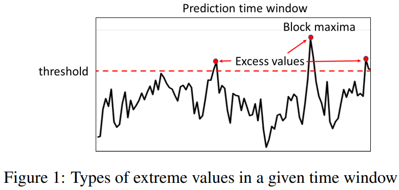
The two most popular distributions studied in EVT are the generalized extreme value (GEV) and generalized Pareto (GP) distributions. Given a prediction time window, GEV governs the distribution of its block maxima, whereas GP is concerned with the distribution of excess values over a certain threshold.
This paper focuses on forecasting the block maxima as it allows us to assess the worst-case scenario in the given forecast time window and avoids making ad-hoc decisions regarding the choice of excess threshold to use for the GP distribution.
Deep learning methods have grown in popularity in recent years due to their ability to capture nonlinear dependencies in the data. Previous studies have utilized a variety of deep neural network architectures for time series modeling. However, these works are mostly focused on predicting the conditional mean of the target variable.

While there have some recent attempts to incorporate EVT into deep learning they are primarily focused on modeling the tail distribution, i.e., excess values over a threshold, using the GP distribution, rather than forecasting the block maxima using the GEV distribution.
Incorporating the GEV distribution into the deep learning formulation presents many technical challenges. First, the GEV parameters must satisfy certain positivity constraints to ensure that the predicted distribution has a finite bound. Another challenge is the scarcity of data since there is only one block maximum value per time window. This makes it hard to accurately infer the GEV parameters for each window from a set of predictors. Finally, the training process is highly sensitive to model initialization. For example, the random initialization of a deep neural network (DNN) can easily violate certain regularity conditions of the GEV parameters estimated using maximum likelihood (ML) estimation.
To overcome these challenges, the authors propose a novel framework called DeepExtrema that utilizes the GEV distribution to characterize the distribution of block maximum values for a given forecast time window. The parameters of the GEV distribution are estimated using a DNN, which is trained to capture the nonlinear dependencies in the time series data.
- The authors present a novel framework to predict the block maxima of a given time window by incorporating GEV distribution into the training of a DNN.
- The authors propose a reformulation of the GEV constraints to ensure they can be enforced using activation functions in the DNN.
- The authors introduce a model bias offset mechanism to ensure that the DNN output preserves the regularity conditions of the GEV parameters despite its random initialization.
- The authors perform extensive experiments on both real-world and synthetic data to demonstrate the effectiveness of DeepExtrema compared to other baseline methods.
Preliminaries Link to heading
Problem Statement Link to heading
Let $z_1, z_2, \cdots, z_T$ be a time series of length $T$. Assume the time series is partitioned into a set of time windows, where each window $[t-\alpha, t+\beta]$ contains a sequence of predictors, $x_t=\left(z_{t-\alpha}, z_{t-\alpha+1}, \cdots, z_t\right)$, and target, \(\tilde{y}_t=\left(z_{t+1}, z_{t+2}, \cdots, z_{t+\beta}\right)\). Note that $\beta$ is known as the forecast horizon of the prediction. For each time window, let $y_t=\max_{\tau \in{1, \cdots, \beta}} z_{t+\tau}$ be the block maxima of the target variable at time $t$. Our time series forecasting task is to estimate the block maxima, \(\hat{y}_t\), as well as its upper and lower quantile estimates, \(\hat{y}_{U}\) and \(\hat{y}_{L}\), of a future time window based on current and past data, $x_t$.
Generalized Extreme Value Distribution Link to heading
The GEV distribution governs the distribution of block maxima in a given window. Let \(Y=\max\left\{z_1, z_2, \cdots, z_t\right\}\). If there exist sequences of constants $a_t>0$ and $b_t$ such that
$$ \operatorname{Pr}\left(Y-b_t\right) / a_t \leq y \rightarrow G(y) \quad \text { as } t \rightarrow \infty $$for a non-degenerate distribution $G$, then the cumulative distribution function $G$ belongs to a family of GEV distribution of the form [Coles et al., 2001]:
$$ G(y)=\exp \left\{-\left[1+\xi\left(\frac{y-\mu}{\sigma}\right)\right]^{-1 / \xi}\right\} \tag{1} $$The GEV distribution is characterized by the following parameters: $\mu$ (location), $\sigma$ (scale), and $\xi$ (shape). The expected value of the distribution is given by
$$ y_{\text {mean }}=\mu+\frac{\sigma}{\xi}[\Gamma(1-\xi)-1] \tag{2} $$where $\Gamma(x)$ denotes the gamma function of a variable $x>0$. Thus, $y_{\text {mean }}$ is only well-defined for $\xi<1$. Furthermore, the $p^{t h}$ quantile of the GEV distribution, $y_p$, can be calculated as follows:
$$ y_p=\mu+\frac{\sigma}{\xi}\left[(-\log p)^{-\xi}-1\right] \tag{3} $$Given $n$ independent block maxima values, \(\left\{y_1, y_2, \cdots, y_n\right\}\), with the distribution function given by Equation (1) and assuming $\xi \neq 0$, its log-likelihood function is given by:
$$ \ell_{G E V}(\mu, \sigma, \xi)= -n \log \sigma-\left(\frac{1}{\xi}+1\right) \sum_{i=1}^n \log \left(1+\xi \frac{y_i-\mu}{\sigma}\right) -\sum_{i=1}^n\left(1+\xi \frac{y_i-\mu}{\sigma}\right)^{-1 / \xi} \tag{4} $$The GEV parameters $(\mu, \sigma, \xi)$ can be estimated using the maximum likelihood (ML) approach by maximizing (4) subject to the following positivity constraints:
$$ \sigma>0 \quad \text { and } \quad \forall i: 1+\frac{\xi}{\sigma}\left(y_i-\mu\right)>0 \tag{5} $$In addition to the above positivity constraints, the shape parameter $\xi$ must be within certain range of values in order for the ML estimators to exist and have regular asymptotic properties. Specifcally, the ML estimators have regular asymptotic properties as long as $\xi > −0.5$. Otherwise, if $−1 < \xi < −0.5$, then the ML estimators may exist but will not have regular asymptotic properties. Finally, the ML estimators do not exist if $\xi < −1$

DeepExtrema Link to heading
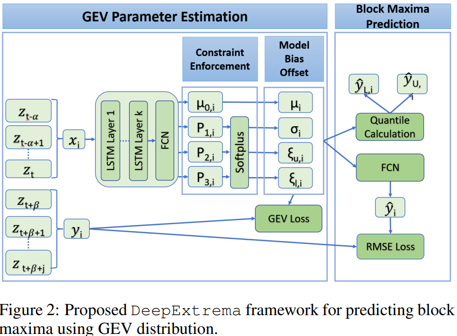
The predicted block maxima $\hat{y}$ follows a GEV distribution, whose parameters are conditioned on observations of the predictors $x$. Given the input predictors $x$, the framework uses a stacked LSTM network to learn a representation of the time series. The LSTM will output a latent representation, which will used by a fully connected layer to generate the GEV parameters
$$ (\mu, \sigma, \xi_{u}, \xi_{l}) = LSTM(x) \tag{6} $$where $\mu$, $\sigma$, and $\xi$’s are the location, shape, and scale parameters of the GEV distribution.
The proposed Model Bias Offset (MBO) component performs bias correction on the estimated GEV parameters to ensure that the LSTM outputs preserve the regularity conditions of the GEV parameters irrespective of how the network was initialized. The GEV parameters are subsequently provided to a fully connected layer to obtain point estimates of the block maxima, which include its expected value yˆ as well as upper and lower quantiles, \(\hat{y}_{U}\) and \(\hat{y}_{L}\).
The GEV parameters are then used to compute the negative log-likelihood of the estimated GEV distribution, which will be combined with the root-mean-square error (RMSE) of the predicted block maxima to determine the overall loss function.
GEV Parameter Estimation Link to heading
Let \(D = \{(x_{i}, y_{i})\}_{n}^{i=1}\) be a set of training examples, where each $x_{i}$ denotes the predictor time series and $y_{i}$ is the corresponding block maxima for time window $i$.
A naıve approach is to assume that the GEV parameters $(\mu, \sigma, \xi)$ are constants for all time windows. This can be done by fitting a global GEV distribution to the set of block maxima values $y_{i}$’s using the maximum likelihood approach.
Instead of using a global GEV distribution with fixed parameters, our goal is to learn the parameters $(\mu_{i}, \sigma_{i}, \xi_{i})$ of each window $i$ using the predictors $x_{i}$.
The estimated GEV parameters generated by the LSTM must satisfy the two positivity constraints given by the inequalities in (5). While the frst positivity constraint on $\sigma_{i}$ is straightforward to enforce, maintaining the second one is harder as it involves a nonlinear relationship.
The authors propose a reformulation of the second constraint in (5). This allows the training process to proceed even though the second constraint in (5) has yet to be satisfed especially in the early rounds of the training epochs. Specifcally, we relax the hard constraint by adding a small tolerance factor, $\tau > 0$
$$ \forall i: 1 + \frac{\xi}{\sigma}(y_{i} - \mu) + \tau \ge 0 \tag{7} $$The preceding soft constraint allows for minor violations of the second constraint in (5) as long as (7) hold for all time windows $i$.
Assuming $\xi \neq 0$, the soft constraint in (7) can be reformulated into the following bounds on $\xi$ :
$$ -\frac{\sigma}{y_{\max }-\mu}(1+\tau) \leq \xi \leq \frac{\sigma}{\mu-y_{\min }}(1+\tau) $$where $\tau$ is the tolerance on the constraint in (5).
The upper and lower bound constraints on $\xi$ in (8) can be restated as follows:
$$ \begin{aligned} & \frac{\sigma}{\mu-y_{\min }}(1+\tau)-\xi \geq 0 \\ & \xi+\frac{\sigma}{y_{\max }-\mu}(1+\tau) \geq 0 \end{aligned} $$Given an input $x_i$, DeepExtrema will generate the following four outputs: $\mu_i, P_{1 i}, P_{2 i}$, and $P_{3 i}$. A softplus activation function, $\operatorname{softplus}(x)=\log (1+\exp (x))$, which is a smooth approximation to the $ReLU$ function, is used to enforce the non-negativity constraints associated with the GEV parameters.
The scale parameter $\sigma_i$ can be computed using the softplus activation function on $P_{1 i}$ as follows:
$$ \sigma_i=\operatorname{softplus}\left(P_{1 i}\right) $$This ensures the constraint $\sigma_i \geq 0$ is met. The lower and upper bound constraints on $\xi_i$ given by the inequalities in (9) are enforced using the softplus function on $P_{2 i}$ and $P_{3 i}$ :
$$ \begin{aligned} & \frac{\sigma_i}{\mu_i-y_{\min }}(1+\tau)-\xi_{u, i}=\operatorname{softplus}\left(P_{2 i}\right) \\ & \frac{\sigma_i}{y_{\max }-\mu_i}(1+\tau)+\xi_{l, i}=\operatorname{softplus}\left(P_{3 i}\right) \end{aligned} $$By re-arranging the above equation, we obtain
$$ \begin{aligned} \xi_{u, i} & =\frac{\sigma_i}{\mu_i-y_{\min }}(1+\tau)-\operatorname{softplus}\left(P_{2 i}\right) \\ \xi_{l, i} & =\operatorname{softplus}\left(P_{3 i}\right)-\frac{\sigma_i}{y_{\max }-\mu_i}(1+\tau) \end{aligned} $$The MLestimated distribution may not have the asymptotic GEV distribution when $\xi < −0.5$ while its conditional mean is not well-defned when $\xi > 1$. Additionally, the estimated location parameter µ may not fall within the desired range between $y_{\text{min}}$ and $y_{\text{max}}$ when the DNN is randomly initialized
One way to address this challenge is to repeat the random initialization of the DNN until a reasonable set of initial GEV parameters, i.e., $y_{\text{min}} \le \mu \le y_{\text{max}}$ and $−0.5 < \xi < 1$, is found.

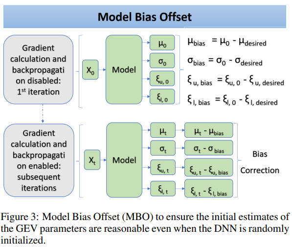
The authors introduce a simple but effective technique called Model Bias Offset (MBO) to address this challenge. The key insight here is to view the GEV parameters as a biased output due to the random initialization of the DNN and then perform bias correction to alleviate the effect of the initialization
To do this, let $\mu_{\text{desired}}$, $\sigma_{\text{desired}}$, and $\xi_{\text{desired}}$ be an acceptable set of initial GEV parameters. The values of these initial parameters must satisfy the regularity conditions $−0.5 < \xi_{\text{desired}}< 1$, $\sigma_{\text{desired}} > 0$, and $y_{\text{min}} \le \mu_{\text{desired}} \le y_{\text{min}}$.
When the DNN is randomly initialized, let $\mu_{0}$, $\sigma_{0}$, $\xi_{u,0}$, and $\xi_{l,0}$ be the initial DNN output for the GEV parameters. These initial outputs may not necessarily fall within their respective range of acceptable values.
$$ \begin{aligned} \mu_{\text {bias }}=\mu_0-\mu_{\text {desired }} \\ \sigma_{\text {bias }}=\sigma_0-\sigma_{\text {desired }} \\ \xi_{u, \text { bias }}=\xi_{u, 0}-\xi_{u, \text { desired }} \\ \xi_{l, \text { bias }}=\xi_{l, 0}-\xi_{l, \text { desired }} \end{aligned} \tag{14} $$The model bias terms in (14) can be computed during the initial forward pass of the algorithm. The gradient calculation and back-propagation are disabled during this step to prevent the DNN from computing the loss and updating its weight with the unacceptable GEV parameters.
$$ \begin{aligned} \mu_t \rightarrow \mu_t-\mu_{\text {bias }} \\ \sigma_t \rightarrow \sigma_t-\sigma_{\text {bias }} \\ \xi_{u, t} \rightarrow \xi_{u, t}-\xi_{u, \text { bias }} \\ \xi_{l, t} \rightarrow \xi_{l, t}-\xi_{l, \text { bias }} \end{aligned} \tag{15} $$Block Maxima Prediction Link to heading
Given an input $x_{i}$, the DNN will estimate the GEV parameters needed to compute the block maxima \(\hat{y}_{i}\) along with its upper and lower quantiles, \(\hat{y}_{U,i}\) and \(\hat{y}_{L,i}\), respectively. The quantiles are estimated using the formula given in (3).
The loss function to be minimized by DeepExtrema
$$ \mathcal{L} = \lambda_{1}\hat{\mathcal{L}} + (1-\lambda_{1})\sum_{i=1}^{n}(y_{i}-\hat{y}_{i})^{2} $$where $\hat{\mathcal{L}} = -\lambda_{2} \ell_{GEV} (\mu, \sigma, \xi)+ (1-\lambda_{2})\sum_{i=1}^{n}(\xi_{u,i} −\xi_{l,i})^{2}$ is the regularized GEV loss.
The first term in $\hat{\mathcal{L}}$ corresponds to the negative log-likelihood function given in Equation (4) while the second term minimizes the difference between the upper and lower-bound estimates of $\xi$.