Abstract Link to heading
Recent deep learningbased methods overlook the existence of extreme events, which result in weak performance when applying them to real time series. Extreme events are rare and random, but do play a critical role in many real applications, such as the forecasting of financial crisis and natural disasters. In this paper, the authors explore the central theme of improving the ability of deep learning on modeling extreme events for time series prediction.
The authors first find that the weakness of deep learning methods roots in the conventional form of quadratic loss. To address this issue, the authors take inspirations from the Extreme Value Theory, developing a new form of loss called Extreme Value Loss (EVL) for detecting the future occurrence of extreme events. Furthermore, the authors propose to employ Memory Network in order to memorize extreme events in historical records.
Introduction Link to heading
Most previously studied DNN are observed to have troubles in dealing with data imbalance Following the discussion in Lin et al., such an imbalance in data will potentially bring any classifier into either of two unexpected situations: a. the model hardly learns any pattern and simply chooses to recognize all samples as positive. b. the model memorizes the training set perfectly while it generalizes poorly to test set.
In the context of time-series prediction, imbalanced data in time series, or extreme events, is also harmful to deep learning models. Intuitively, an extreme event intime series is usually featured by extremely small or large values, of irregular and rare occurrences.
As an empirical justification of its harmfulness on deep learning models, the authors train a standard GRU to predict one-dimensional time series, where certain thresholds are used to label a small proportion of datasets as extreme events in prior.
a. In Fig. 1(a), most of its predictions are bounded by thresholds and therefore it fails to recognize future extreme events, the authors claim this as underfitting phenomenon. b. In Fig. 1(b), although the model learns extreme events in the train set correctly, it behaves poorly on test sets, the authors cliam this as overfitting phenomenon
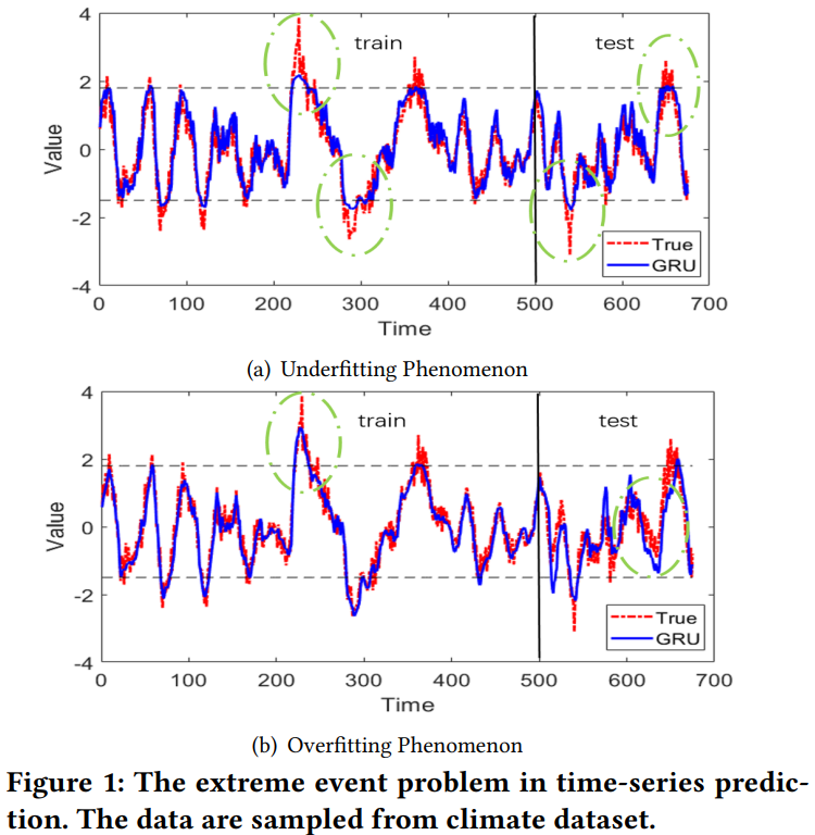
However from the authors’ perspective, it would be really valuable if a time-series prediction model could recognize future extreme events with reasonable predictions.
- We provide a formal analysis on why deep neural network suffers underfitting or overfitting phenomenons during predicting time series data with extreme value
- We propose a novel loss function called Extreme Value Loss (EVL) based on extreme value theory, which provides better predictions on future occurrences of extreme events.
- We propose a brand-new Memory Network based neural architecture to memorize extreme events in history for better predictions of future extreme values. Experimental results validates the superiority of our framework in prediction accuracy compared with the state-of-the-arts.
Preliminaries Link to heading
Time Series Prediction Link to heading
Suppose there are $N$ sequences of fixed length $T$. For the $i$-th sequence the time series data can be described as
$$ \left(X_{1: T}^{(i)}, Y_{1: T}^{(i)}\right)=\left[\left(x_1^{(i)}, y_1^{(i)}\right),\left(x_2^{(i)}, y_2^{(i)}\right), \cdots,\left(x_T^{(i)}, y_T^{(i)}\right)\right] $$where $x_t^{(i)}$ and $y_t^{(i)}$ are input and output at time $t$ respectively. In one-dimensional time series prediction the authors have $x_t^{(i)}, y_t^{(i)} \in \mathbb{R}$ and $y_t^{(i)}:=x_{t+1}^{(i)}$. For the sake of convenience, the authors will use $X_{1: T}=$ $\left[x_1, \cdots, x_T\right]$ and $Y_{1: T}=\left[y_1, \cdots, y_T\right]$ to denote general sequences without referring to specific sequences.
The goal of time-series prediction is that, given observations $\left(X_{1: T}, Y_{1: T}\right)$ and future inputs $X_{T: T+K}$, how to predict outputs $Y_{T: T+K}$ in the future. Suppose a model predicts $o_t$ at time $t$ given input $x_t$, the common optimization goal can be written as,
$$ \min \sum_{t=1}^T\left\|o_t-y_t\right\|^2 $$Then after the inference the model could predict the corresponding outputs $O_{1: T+K}$ give inputs $X_{1: T+K}$.
Extreme Events Link to heading
Although DNN such as GRU has achieved noticeable improvements in predicting time-series data, this model tends to fall into either overfitting or underfitting if trained with imbalanced time series as Extreme Event Problem.
It will be convenient to introduce an auxiliary indicator sequenc $V_{1:T} = [v_{1}, \ldots, v_{T}]$
$$ v_{t} = \begin{cases}1 \quad y_{t} > \epsilon_{1} \\ 0 \quad y_{t} \in [-\epsilon_{2}, \epsilon_{1}] \\ -1 \quad y_{t} < -\epsilon_{2} \end{cases} $$where large constants $\epsilon_{1}$, $\epsilon_{2} > 0$ are called thresholds. For time step $t$, if $v_{t} = 0$, the authors define the output $y_{t}$ as normal event. If $v_{t} > 0$, the authors define the output $y_{t}$ as right extreme event. If $v_{t} < 0$, the authors define the output $y_{t}$ as left extreme event.
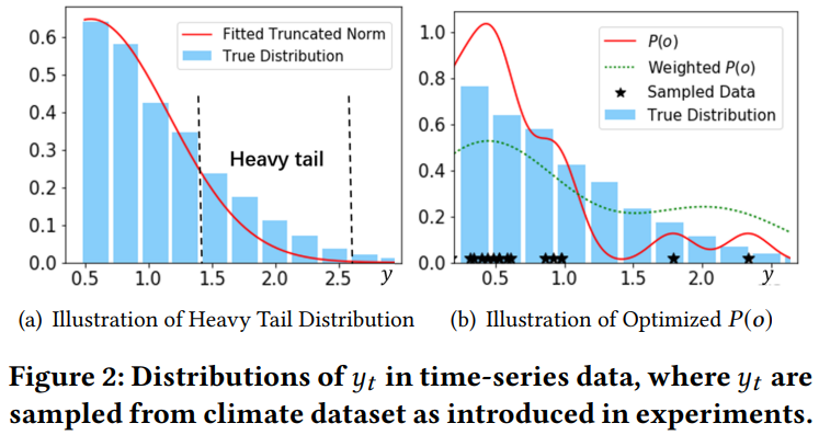
Heavy-tailed. If a random variable $Y$ is said to respect a heavy-tailed distribution, then it usually has a non-negligible probability of taking large values (larger than a threshold. A majority of widely applied distributions including Gaussian, Poisson are not heavy-tailed, therefore, light-tailed.
Only a few number of parametric distributions are heavy-tailed, e.g. Pareto distribution and log-Cauchy distribution. Therefore modeling with light-tailed parametric distributions would bring unavoidable losses in the tail part of the data.
Extreme Value Theory. EVT studies the distribution of maximum in observed samples [43]. Formally speaking, suppose $T$ random variables $y_{1}, \ldots ,y_{T}$ are i.i.d sampled from distribution $F_{Y}$, then the distribution of the maximum is
$$ \text{lim}_{T\rightarrow\infty} P\{\text{max}(y_{1}, \ldots, y_{T}) \leq y\} = \text{lim}_{T\rightarrow\infty} F^{T}(y) = 0 $$In order to obtain a non-vanishing form of $P{\text{max}(y_{1},\ldots,y_{T}) \leq y}$, previous researches proceeded by performing a linear transformation on the maximum.
If there exists a linear transformation on $Y$ which makes the distribution non-degenetated to 0. Then the class of the non-degenerated distribution $G(y)$ after the transformation must be the following distribution:
$$ G(y) = \begin{cases} \exp(-(1-\frac{1}{\gamma}y)^{\gamma}), \quad \gamma \neq 0, 1 - \frac{1}{\gamma}y > 0 \\ \exp(-e^{-y}), \quad \gamma = 0 \end{cases} $$Usually, the form $G(y)$ is called Generalized Extreme Value distribution, with $\gamma$, $0$ as extreme value index.
Modeling The Tail. Previous works extend the above theorem to model the tail distribution
$$ 1 - F(y) \approx (1 - F(\xi))\left[1 - \log G \left(\frac{y-\xi}{f(\xi)}\right)\right], y > \xi $$where $\xi > 0$ is a sufficiently large threshold.
Problems caused by Extreme Events Link to heading
Empirical Distribution After Optimization Link to heading
From the probabilistic perspective, minimization of the loss function in Eq. 2 is in essence equivalent to the maximization of the likelihood $P(y_{t}|x_{t})$. Based on Bregman’s theory, minimizing such square loss always has the form of Gaussian with variance $\tau$, that is, $p(y_{t}|x_{t}, \theta) = \mathcal{N} (o_{t}, \tau^{2})$, where $\theta$ is the parameter of the predicting model, $\mathbf{O}_{1:T}$ are outputs from the model.
Eq. 2 can be replaced with its equivalent optimization problem as follow
$$ \text{max}_{\theta} \prod_{t=1}^{T}P(y_{t}|x_{t}, \theta) $$With Bayes’s theorem, the likelihood above can be written as,
$$ P(Y|X) = \frac{P(X|Y)P(Y)}{P(X)} $$By assuming the model has sufficient learning capacity with parameter $\theta$, the inference problem will yield an optimal approximation to $P(Y|X)$. if $P(Y|X)$ has been perfectly learned, so as the distributions $P(Y)$, $P(X)$, $P(X|Y)$, which are therefore totally independent of inputs $X$. By considering the following observations
- The discriminative model has no prior on $y_{t}$
- The output $o_{t}$ is learned under likelihood as normal distribution it is therefore reasonable to state that empirical distribution $P(Y)$ after optimization should be of the following form
where constant $\hat{\tau}$ is an unknown variance. In consideration of its similarity to Kernel Density Estimator (KDE) with Gaussian Kernel the authors can reach an intermediate conclusion that such a model would perform relatively poor if the true distribution of data in series is heavy-tailed.
Why Deep Neural Network Could Suffer Extreme Event Problem Link to heading
The distribution of output from a learning model with optimal parameters can be regarded as a KDE with Gaussian Kernel. Since nonparametric kernel density estimator only works well with sufficient samples, the performance therefore is expected to decrease at the tail part of the data, where sampled data points would be rather limited.
The main reason is that the range of extreme values are commonly very large, thus few samples hardly can cover the range.
Suppose $x_{1}$, $x_{2}$ are two test samples with corresponding outputs as $o_{1} = 0.5$, $o_{2} = 1.5$. As our studied model is assumed to have sufficient learning capacity for modeling $P(X)$, $P(X|Y)$, thus the authors have
$$ P(y_{1}|x_{1},\theta) = \frac{P(X|Y)\hat{P}(Y)}{P(X)} \ge \frac{P(X|Y)P_{\text{true}}(Y)}{P(X)} = P_{\text{true}}(y_{1}|x_{1}) $$Similarly $P(y_{2}|x_{2},\theta) ≤ P_{\text{true}}(y_{2}|x_{2})$. Therefore, in this case, the predicted value from deep neural network are always bound, which immediately disables deep model from predicting extreme events, i.e. causes the underfitting phenomenon.
On the other side, several methods propose to accent extreme points during the training by, for example, increasing the weight on their corresponding training losses. these methods are equivalent to repeating extreme points for several times in the dataset when fitting KDE
$$ P(y_{2}|x_{2},\theta) = \frac{P(X|Y)\hat{P}(Y)}{P(X)} \ge \frac{P(X|Y)P_{\text{true}}(Y)}{P(X)} = P_{\text{true}}(y_{2}|x_{2}) $$The inequality above indicates, with the estimated probability of extreme events being added up, the estimation of normal events would simultaneously become inaccurate. Therefore, normal data in the test set is prone to be mis-classified as extreme events, which therefore marks the overfitting phenomenon.
Predicting Time Series Data with Extreme Events Link to heading
In order to impose prior information on tail part of observations for DNN, the authors focus on two factors: memorizing extreme events and modeling tail distribution.
For the first factor, the authors use memory network to memorize the characteristic of extreme events in history, and for the latter factor the authors propose to impose approximated tailed distribution on observations and provide a novel classification called Extreme Value Loss (EVL)
Memory Network Module Link to heading
Extreme events in time-series data often show some form of temporal regularity. The authors propose to use memory network to memorize these extreme events, which is proved to be effective in recognizing inherent patterns contained in historical information.
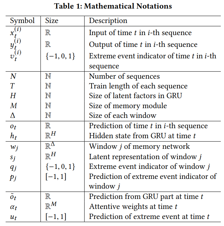
Historical Window. For each time step $t$, first, the authors randomly sample a sequence of windows by $W = {w_{1}, \ldots, w_{M}}$, where $M$ is the size of the memory network. Each window $w_{j}$ is formally defined as $w_{j} = [x_{t_{j}}, x_{t_{j}+1},\ldots, x_{t_{j}+\Delta}]$, where $\Delta$ as the size of the window satisfying $0 < t_{j} < t − \Delta$.
Then, the authors apply GRU module to embed each window into feature space. Specifically, the authors use $w_{j}$ as input, and regard the last hidden state as the latent representation of this window, denoted as $s_{j} = \mathrm{GRU}([x_{t_{j}}, x_{t_{j}+1},\ldots, x_{t_{j}+\Delta}]) ∈ \mathbb{R}^{H}$.
Meanwhile, the authors apply a memory network module to memorize whether there is a extreme event in $t_{j}+\Delta+1$ for each window $w_{j}$. In implementation, the authors propose to feed the memory module by $q_{j} = v_{t_{j}+\Delta+1} \in {−1, 0, 1}$.
In summary, at each time step $t$, the memory consists of the following two parts: -Embedding Module $S \in \mathbb{R}^{M \times H}: s_{j}$ is the latent representation of history window $j$. -History Module $Q \in {−1, 0, 1}^{M} : q_{j}$ is the label of whether there is a extreme event after the window $j$.
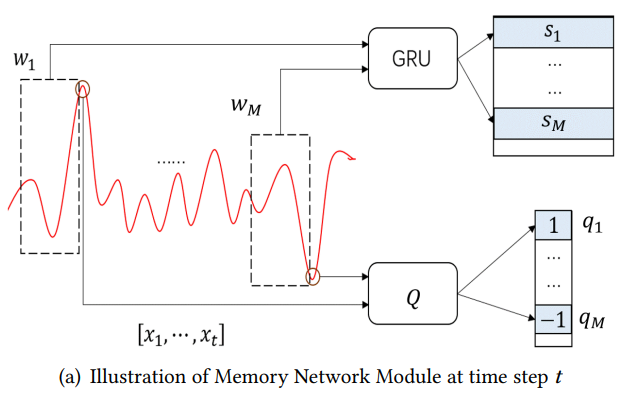
Attention Mechanism.. At each time step $t$, the authors use GRU to produce the output value
$$ \tilde{o}_{t} = W_{o}^{\top}h_{t}+b_{o} \text{ where } h_{t} = \mathrm{GRU}([x_{1}, x_{2}, \ldots, x_{t}]) $$where $h_{t}$ and $s_{j}$ share the same GRU units.
The prediction of o˜t may lack the ability of recognizing extreme events in the future. This requires our model to retrospect its memory to check whether there is a similarity between the target event and extreme events in history. To do that, the authors propose to utilize attention mechanism
$$ \alpha_{tj} = \frac{\exp(c_{tj})}{\sum_{j=1}^{M}\exp(c_{tj})}, \text{ where } c_{tj} = h_{t}^{\top}s_{j} $$Finally, the prediction of whether an extreme event would happen after referring historical information can be measured by imposing attentive weights on $q_{j}$. The output at time step $t$ is calculated as
$$ o_{t} = \tilde{o}_{t} + b^{\top}u_{t}, \text{ where } u_{t} = \sum_{j=1}^{M}\alpha_{tj}q_{j} $$$u_{t} \in [−1, 1]$ is the prediction of whether there will be an extreme event after time step $t$, and \(b \in \mathbb{R}_{+}\) is the scale parameter. When there is a similarity between the current time step and certain extreme events in history, then ut will help detect such a pumping point by settingut non-vanishing, while when the current event is observed to hardly have any relation with the history, then the output would choose to mainly depend on $\tilde{o}_{t}$, i.e. the value predicted by a standard GRU gate
Extreme Value Loss Link to heading
Although memory network could forecast some extreme events, such loss function still suffer extreme events problem. In order to incorporate the tail distribution with $P(Y)$, the authors first consider the approximation. The approximation can be written as
$$ 1 - F(y_{t}) \approx (1 - P(v_{t} = 1))\log G \left(\frac{y_{t}-\epsilon_{1}}{f(\epsilon_{1})}\right) $$where positive function $f$ is the scale function. The predicted indicator is $u_{t}$, which can be regarded as a hard approximation for $(y_{t} − \epsilon_{1})/f (\epsilon_{1})$.
The authors regard the approximation as weights and add them on each term in binary cross entropy
$$ \begin{aligned} \operatorname{EVL}\left(u_t\right)= & -\left(1-P\left(v_t=1\right)\right)\left[\log G\left(u_t\right)\right] v_t \log \left(u_t\right) \\ & -\left(1-P\left(v_t=0\right)\right)\left[\log G\left(1-u_t\right)\right]\left(1-v_t\right) \log \left(1-u_t\right) \\ = & -\beta_0\left[1-\frac{u_t}{\gamma}\right]^\gamma v_t \log \left(u_t\right) \\ & -\beta_1\left[1-\frac{1-u_t}{\gamma}\right]^\gamma\left(1-v_t\right) \log \left(1-u_t\right) \end{aligned} $$where $\beta_{0} = P(v_{t} = 0)$, which is the proportion of normal events in the dataset and $P(v_{t} = 1)$ is the proportion of right extreme events in the dataset. $\gamma$ is the hyper-parameter, which is the extreme value index in the approximation. Similarly the authors have the binary classification loss function for detecting whether there will be a left extreme event in the future. Combining two loss functions together the authors can extend EVL to the situation of $v_{t} = {−1, 0, 1}$
:::warning The key point of EVL is to find the proper weights by adding approximation, e.g., $\beta_{0}[1 − u_{t}/\gamma]^{\gamma}$, on tail distribution of the observations through extreme value theory. Intuitively, for detecting right extreme event, term $\beta_{0}$ will increase the penalty when the model recognizes the event as normal event. Meanwhile, the term $[1 − u_{t}/\gamma]^{\gamma}$ also increase the penalty when the model recognize the extreme event with little confidence :::
Optimization Link to heading
To incorporate EVL with the proposed memory network, a direct thought is to combine the predicted outputs ot with the prediction of the occurrence of extreme event
$$ L_{1} = \sum_{t=1}^{T}||o_{t}-y_{t}||^{2} + \lambda_{1} EVL(u_{t}, v_{t}) $$To enhance the performance of GRU units, the authors propose to add the penalty term for each window $j$, which aims at predicting extreme indicator $q_{j}$ of each window $j$
$$ L_{2} = \sum_{t=1}^{T}\sum_{j=1}^{M}EVL(p_{j},q_{j}) $$where $p_{j} \in [−1, 1]$ is calculated through $s_{j}$, which is the embedded representation of window $j$, by a full connection layer.
Experiments Link to heading

