Abstract Link to heading
Deep learning methods have achieved state-of-the-art performance in anomaly detection in recent years; unsupervised methods being particularly popular. However, deep learning methods can be fragile to small perturbations in the input data. This phenomena has been widely studied in the context of supervised image classification since its discovery, however such studies for an anomaly detection setting are sorely lacking. Moreover, the plethora of defense mechanisms that have been proposed are often not applicable to unsupervised anomaly detection models
Introduction Link to heading
Anomaly is observations which deviates so much from other observations as to arouse suspicion it was generated by a different mechanism.
Recently, deep learning methods have given the best performance; particularly popular is to train an autoencoder to reconstruct data of the normal class, using the reconstruction error to determine whether a point is anomalous.
Despite their successes, the highly complex operations of deep learning models can make their outputs fragile to small perturbations in input data. This makes them vulnerable to an adversary who may exploit perturbations that are purpose- fully designed to greatly hinder model performance.
A number of defense mechanisms have been devised against adversarial attacks which is ‘adversarial training’. This introduces data that has been perturbed with an adversarial attack into the training set along with their correct labels.
In the case of unsupervised anomaly detection, no labels are supplied to the model and anomalies are only seen during test time, meaning this defense is inapplicable.
Background Link to heading
Anomaly Detection with Autoencoders Link to heading
Autoencoders are neural networks that are trained to reconstruct the input data, with the error between the original and the reconstruction
$$ \tag{1} \mathrm{err}(\mathbf{x}) = || \mathbf{x} - \mathrm{AE}(\mathbf{x}) || $$where \(\mathbf{x}\) and \(\mathrm{AE}(\mathbf{x})\) is the input and output of the autoencoder respectively and \(|| \cdot ||\) is typically some type of norm.
Adversarial Attack Link to heading
The input data can be perturbed as to hinder model performance through adversarial attacks. In fast gradient sign method (FGSM) inputs are moved in the direction of the gradient of the loss function to increase the loss function with respect to the true class and encourage a misclassification.
$$ \tag{2} \mathbf{x}_{0}^{\text{adv}} = \mathbf{x}\\ \mathbf{x}_{t+1}^{\text{adv}} = \mathrm{clip}_{\mathbf{x}, \epsilon}\{\mathbf{x}_{t}^{\text{adv}} + \alpha \cdot \mathrm{sign}(\nabla_{\mathbf{x}}(\mathcal{L}(\mathbf{x}_{t}^{\text{adv}}, y_{\text{true}})))\} $$Related Work Link to heading
Unsupervised versions of anomaly detection algorithms have been developed, most notably the One-class SVM and LOF. The non-linearity of autoencoders allows for better detection of anomalies than linear PCA, whilst being computationally cheaper than kernel PCA.
Some studies improve the robustness of anomaly detec- tion models to noisy data, such as Robust SVM and Robust PCA. The approach taken in the latter; filtering noise out of input data via matrix decomposition, has also been adopted for autoencoders. However, no similar techniques have been developed in the case of adversarial perturbations.
Methods Link to heading
Attacks Link to heading
Perturbations to anomalous points in the test set that cause the model to misclassify as many of them as possible as normal points. This is achieved by reducing reconstruction error.
Two such attacks are tested: a randomized attack and an FGSM attack.
In the first, a randomly generated vector is added to the original point. If the reconstruction error of this perturbed point is reduced compared to the original, then the perturbation is kept, otherwise it is discarded and another random vector is tested.
In the second, for FGSM he adaptation ensures the reconstruction error i.e. the loss function, decreases rather than increases as follows
$$ \tag{3} \mathbf{x}_{0}^{\text{adv}} = \mathbf{x}\\ \mathbf{x}_{t+1}^{\text{adv}} = \mathbf{x}_{t}^{\text{adv}} - \alpha \cdot \mathrm{sign}(\nabla_{\mathbf{x}}(\mathcal{L}(\mathbf{x}_{t}^{\text{adv}}))) $$Defenses Link to heading
Approximate Projection Link to heading
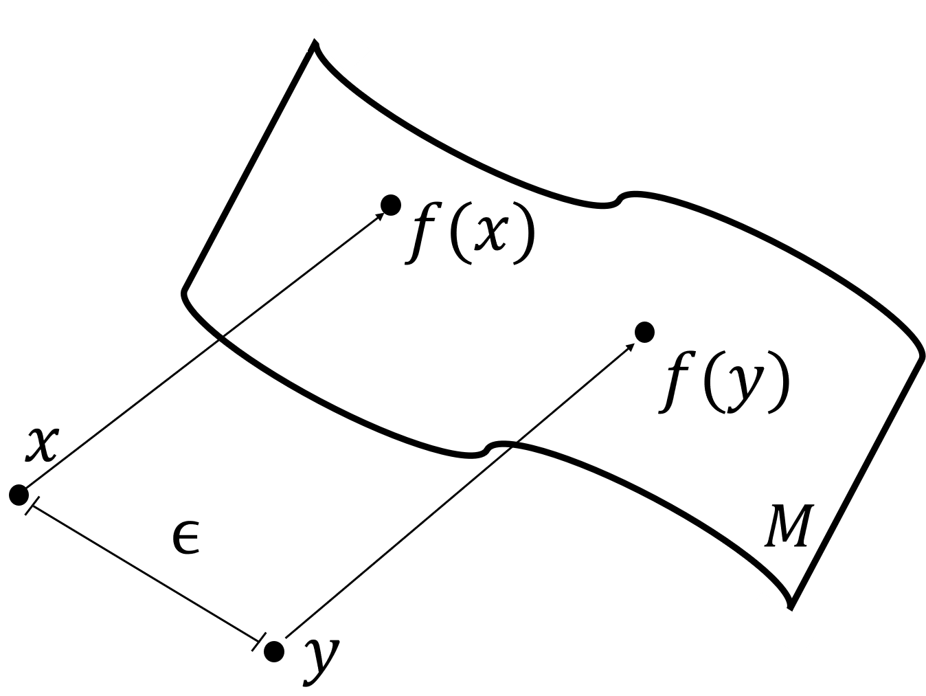 Figure 1: Points \(\mathbf{x}\) and \(\mathbf{y}\) and their projections \(\mathbf{x}'\) and \(\mathbf{y}\), respectively on the image \(\mathcal{M}\).
Autoencoders reconstruct complex data using lower dimensional representations. Adversarial vulnerability can arise because they can learn highly unstable functions that change rapidly in response to small input perturbations.
A class of projection functions which are much more robust is considered.
Formally, let \(A : \mathbb{R}^{d} \rightarrow \mathbb{R}^{d}\) be an autoencoder, and define the image \(\mathcal{M}= \{A(\mathbf{x}) : \mathbf{x} \in \mathbb{R}^{d}\}\) i.e. the set of points that the au- toencoder can map to.
Define the projection \(f(\mathbf{x})\) as the closest point in \(\mathcal{M}\) to \(x\).
$$ f(\mathbf{x}) = \mathrm{arg}\min_{\mathbf{x}' \in \mathcal{M}} ||\mathbf{x} - \mathbf{x}'|| $$Like in autoencoders, the reconstruction error \(\mathrm{err}(x) = ||\mathbf{x}-f(\mathbf{x})||\) is used as an anomaly score.
Theorem 1. If an adversary perturbs a data point from \(\mathbf{x}\) to \(\mathbf{y}\) such that \(||\mathbf{x} - \mathbf{y}|| \leq \epsilon\), then we have:
$$ ||\mathrm{err}(\mathbf{y}) - \mathrm{err}(\mathbf{x})|| \leq \epsilon $$i.e. the adversary can change the reconstruction error of any point \(\mathbf{x}\) by at most $\epsilon$.
Proof. By the triangle inequality we have:
$$ \tag{4} ||\mathbf{x} - f(\mathbf{y})|| \leq ||y - f(\mathbf{x})|| + \epsilon $$\(f(\mathbf{x})\) is the projection of \(\mathbf{x}\) onto \(\mathcal{M}\), therefore, it is the closest point to \(\mathbf{x}\) on \(\mathcal{M}\), so:
$$ \tag{5} ||\mathbf{x} - f(\mathbf{x})|| \leq ||\mathbf{x} - f(\mathbf{y})|| $$Combining this with Equation 4 gives:
$$ \tag{6} ||\mathbf{x} - f(\mathbf{x})|| \leq ||\mathbf{y} - f(\mathbf{y})|| + \epsilon $$or \(\mathrm{err}(x) \leq \mathrm{err}(x) + \epsilon\). By symmetry, the same result holds when swapping \(\mathbf{x}$ and $\mathbf{y}\), completing the proof.
Theorem 1 shows that in the worst-case scenario, an adversary moving a point by \(\epsilon\) distance can decrease the reconstruction error under \(f\) by at most \(\epsilon\). In reality, the projection \(f\) is not accessible as the image \(\mathcal{M}\) is unknown and highly complex.
Instead, after fitting an autoencoder \(A\), we approximate a projection by performing gradient descent on the latent embedding of the data, encoded at the bottleneck layer. Upon convergence, this will lead to a reconstruction that is closer to the optimum; the projection. Gradient descent updates are made via the following formula:
$$ \tag{7} \mathbf{z}_{0} = \mathbf{z} \\ \mathbf{z}_{t+1} = \mathbf{z}_{t} - \alpha * \nabla_{\mathbf{z}}\mathcal{L}(\theta, \mathbf{z}) $$where \(\mathbf{z}\) is the original latent embeddings of test set points under $A$.
Feature Weighting Link to heading
Different features vary in their discriminative capabilities. In particular, regardless of whether points are normal or anomalous, different features tend to be more accurately reconstructed than others through the autoencoder. It is useful to normalize reconstruction error across the different features in order to account for these differences
$$ \hat{J}_{i} = \frac{J_{i}}{\epsilon + \tilde{J}_{i}} $$where \(J_{i}\) is the reconstruction error associated with feature \(i\) for a single point, \(\tilde{J}_{i}\) is the normalizing factor and \(\epsilon\) is a small constant. Various formulations of \(\tilde{J}_{i}\) were considered; the median provides robustness against outliers and good empirical performance. The optimal value of \(\epsilon\) varies between \(10^{-4}\) and \(10^{-6}\) depending on the dataset.
This is a form of normalization which prevents the reconstruction error, and therefore the anomaly score, from being dominated by those features which are reconstructed most poorly regardless of the class.
Whilst improving detection performance, this step alone does not necessarily improve robustness against adversarial attacks. However, in combination with the gradient descent defense, the autoencoder would be more accurate as well as more robust in both the presence and absence of adversarial attacks.
Experiments Link to heading
Datasets Link to heading
| Dataset | #Feature | #Train | #Test | #Anomalies |
|---|---|---|---|---|
| WADI | 1220 | 1,048,571 | 127,792 | 5.99% |
| SWaT | 500 | 496,791 | 449,910 | 11.97% |
Table 1: Summary of the two datasets used in experiments.
Models Link to heading
- APAE: The proposed Approximate Projection Autoencoder
- AE: Autoencoder
- PCA: Principal Component Analysis
- OC-SVM: One-class Support Vector Machine
- DAGMM: Deep Autoencoding Gaussian Mixture Model
- MAD-GAN: Generative Adversarial Networks based Model
Results Link to heading
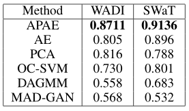 Table 2: AUC score for various anomaly detection methods.
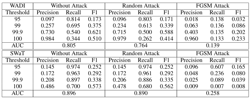 Table 3: Precision, Recall and F1 measures for various anomaly score thresholds for the original test set, the randomly-attacked test set and the FGSM-attacked test set for WADI (top) and SWaT (bottom) datasets
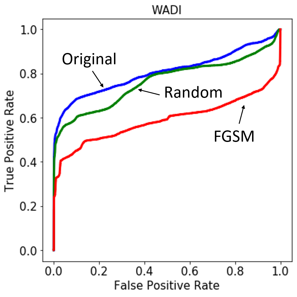
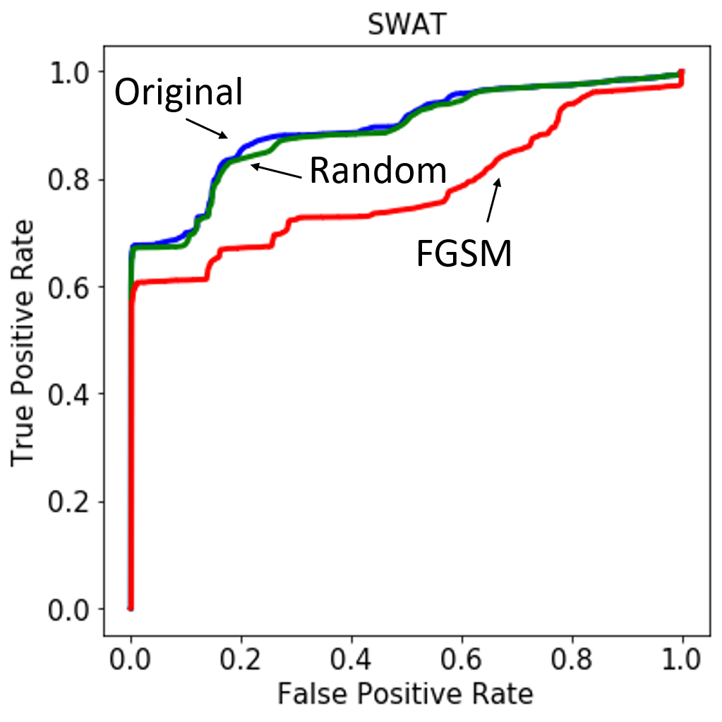 Figure 4: Receiver operating characteristic (ROC) curve for the anomaly-detecting autoencoder on the three test sets used for WADI (left) and SWaT (right).
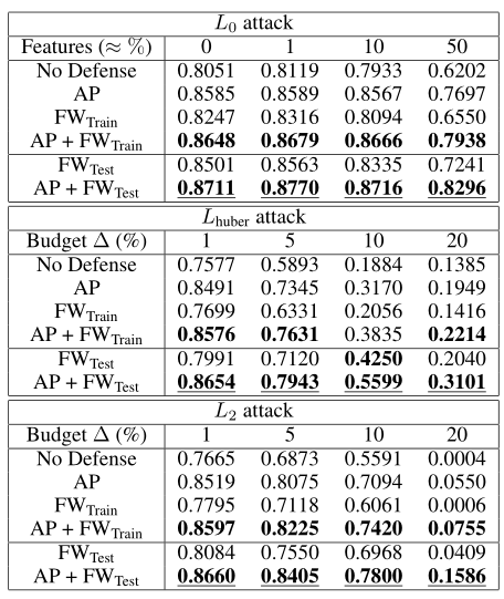 Table 5: WADI: AUC for the three different types of attack with and without defenses.
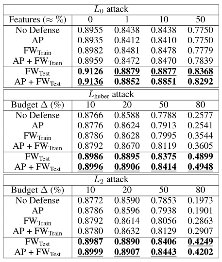 Table 6: SWaT: AUC for the three different types of attack with and without defenses.
Conclusion Link to heading
Deep autoencoders are trained to learn patterns from a set of data of only the normal class. The reconstruction error associated with a point in the test set is used to determine whether it is normal or anomalous. We have considered the context in which an adversary perturbs this data in order to have as many anomalies go undetected as possible. We have shown that the model is indeed vulnerable to this kind of attack, especially to a gradient-based attack like the basic iterative method.