Self-Trained One-class Classification for Unsupervised Anomaly Detection

Abstract Link to heading

In this work, we focus on unsupervised AD problems whose entire training data are unlabeled and may contain both normal and anomalous samples. To tackle this problem, we build a robust one-class classification framework via data refinement. To refine the data accurately, we propose an ensemble of one-class classifiers, each of which is trained on a disjoint subset of training data. Moreover, we propose a self-training of deep representation one-class classifiers (STOC) that iteratively refines the data and deep representations. In experiments, we show the efficacy of our method for unsupervised anomaly detection on benchmarks from image and tabular data domains. For example, with a \(10\%\) anomaly ratio on CIFAR-10 data, the proposed method outperforms state-of-the-art one-class classification method by \(6.3\) AUC and \(12.5\) average precision.

Introduction Link to heading

Figure 1: Anomaly detection problem settings. Blue and red are for labeled negative (normal) and positive (anomalous) samples, respectively. Grey dots denote unlabeled samples. While previous works mostly focus on supervised (a, b) or semi-supervised (c, d, e) settings, we tackle an anomaly detection using only unlabeled data (f) that may contain both negative and positive samples.

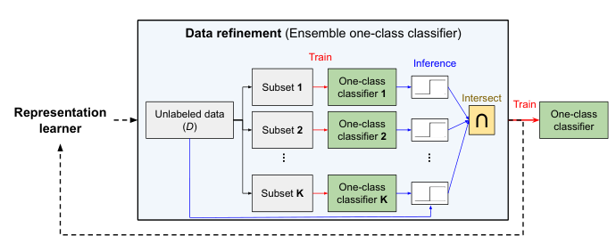
In this paper, we focus on unsupervised anomaly detection problems, where only unlabeled data that may include both negative and positive samples are available during training. Given the impressive performance of one-class classifiers trained on negative samples [20, 23, 5, 41, 28], our goal is to utilize them, and improve their performance by refining the unlabeled training data so as to adopt learning strategies of one-class classification for unsupervised anomaly detection. Inspired by the recent success of self-training in learning without labels [7, 45], we propose a novel self-trained one- class classification (STOC) framework. We illustrate STOC built on a two-stage framework of deep one-class classifiers [41, 28] in Fig. 3. STOC iteratively trains deep representations using refined data while improving refinement of unlabeled data by excluding potential positive (anomalous) samples. For the data refinement process, we employ an ensemble of one-class classifiers, each of which is trained on a different subset of unlabeled training data, and dictate samples as normal with the consensus of all the classifiers. The refined training data are used to train the final one-class classifier to generate the anomaly scores in the unsupervised setting. Unlike previous works [48, 36, 20, 23, 5, 41, 28], STOC works under realistic assumptions that majority of the training data is negative – human labeling can be completely removed from the entire process.

Related Work Link to heading

We review existing works under different settings as described in Fig. 1 and discussed their challenges.

Positive + Negative setting is often considered as a supervised binary classification problem. The challenge arises due to the imbalance in label distributions as positive (anomalous) samples are rare. As summarized in [10], to address this, over-/under-sampling [13, 17], weighted optimization [24, 4], synthesizing data of minority classes [27, 30], and hybrid methods [18, 2] have been studied.

Negative setting is often converted to a one-class classification problem, with the goal of finding a decision boundary that includes as many one-class samples as possible. Shallow models for this setting include one-class support vector machines [38] (OC-SVM), support vector data description [43] (SVDD), kernel density estimation (KDE) [26], and Gaussian density estimation (GDE) [35]. There are also auto-encoder based models [47] that treat the reconstruction error as the anomaly score. In recent years, deep learning based one-class classifiers have been developed, such as deep one- class classifier [36], geometric transformation [20], or outlier exposure [23]. Noting the degeneracy or inconsistency of learning objectives of existing end-to-end trainable deep one-class classifiers, [41] has proposed a deep representation one-class classifier, a two-stage framework that learns self-supervised representations [19, 14] followed by shallow one-class classifiers, and has been extended for texture anomaly localization with CutPaste [28]. The robustness of these methods under unsupervised setting has also been shown in part [48, 5] when the anomaly ratio is very low.

Semi-supervised setting is defined as utilizing small labeled samples and large unlabeled samples to distinguish anomalies from normal data. Depending on which labeled samples are given, we categorize this setting into three sub-categories. If only some positive/negative labeled samples are provided, we denote that as a PU/NU setting. Most previous works in semi-supervised AD settings focused on NU setting where only some of the normal labeled samples are given [34, 42, 1]. PNU setting is a more general semi-supervised setting where subsets of both positive and negative labeled samples are given. Deep SAD [37] and SU-IDS [33] are included in this category. Note that in comparison to Deep SAD, which utilized some labeled data, the proposed framework significantly outperforms under multiple benchmark datasets without using any labeled data (see Section 4.2).

Unlabeled setting has received relatively less attention despite its significance in automating machine learning. Two of the most popular methods for this setting are isolation forest [31] and local outlier factor [11], but they are hard to scale and less compatible with recent advances in representation learning. While one-class classifiers, such as OC-SVM, SVDD, or their deep counterparts, apply to unlabeled settings by assuming the data is all negative, and the robustness of those methods has also been demonstrated in part [48, 5], in practice we observe a significant performance drop with a high anomaly ratio, as shown in Fig. 2. Our proposed framework mostly recovers the lost performance of state-of-the-art shallow and deep one-class classifiers trained on unlabeled data.

Self-training [39, 32] is an iterative training mechanism using machine-generated pseudo labels as targets to train machine learning models. It has regained popularity recently with its successful applications to semi-supervised image classification [7, 40, 45]. Improving the quality of pseudo labels using an ensemble of classifiers is also studied. [12] trains an ensemble of classifiers with different classification algorithms to make a consensus for noisy label verification. Co-training [9] trains multiple classifiers, each of which is trained on the distinct views, to supervised other classifiers. Co-teaching [22] and DivideMix [29] share a similar idea in that they both train multiple deep networks on separate data batches to learn different decision boundaries, thus become useful for noisy label verification. While sharing a similarity, to our knowledge, we are the first to apply self-training to unsupervised learning of an anomaly detector, with no human-generated labels.

Self-Trained One-class Classifier (STOC) Link to heading

Self-Trained One-class Classifier (STOC) is an iterative training method, where we refine the data (Section 3.1) and update the representation with refined data (Section 3.2), followed by building a one-class classifier using refined data and representations, as described in Algorithm 1 and Fig. 3. Note that the framework is amenable to use fixed (e.g., raw or pretrained) representations – in this case, the framework would be composed of a single step of data refinement followed by building an one-class classifier using refined data.

Notation. We denote the training data as \(\mathcal{D} = \{\mathbf{x}_i\}^N_{i=1}\) where \(\mathbf{x}_i \in \mathcal{X}\) and \(N\) is the number of training samples. \(y_i \in \{0, 1\}\) is the corresponding label to \(\mathbf{x}_i\), where \(0\) denotes normal (negative) and \(1\) denotes anomaly (positive). Note that labels are not provided in the unsupervised setting.

Let us denote a feature extractor as \(g : X \rightarrow Z\). \(g\) may include any data preprocessing functions, an identity function (if raw data is directly used for one-class classification), and learned or learnable representation extractors such as deep neural networks. Let us define a one-class classifier as \(f : Z \rightarrow [-\infty, \infty]\) that outputs anomaly scores of the input feature (\(g(\mathbf{x})\)). Higher the score \(f(g(\mathbf{x}))\), more anomalous the sample \(\mathbf{x}\) is, and the binary prediction is made by thresholding: \(\mathbf{1}(f(g(\mathbf{x})) \ge \eta)\).

Data Refinement Link to heading

A naive way to generate pseudo labels of unlabeled data is to construct a one-class classifier on raw or learned representations (e.g., [41]) and threshold the anomaly score to obtain a binary label of normal and anomalous. As we update the model with refined data that excludes samples predicted as positive, it is important to generate pseudo labels of training data as accurately as possible.

Figure 3: Block diagram of STOC composed of representation learner (Section 3.2), data refinement (Section 3.1), and the final one-class classifier blocks. Representation learner updates the deep models using refined data from the data refinement block, but is optional if using fixed representations. Data refinement is done by ensemble one-class classifiers, each of which is trained on K disjoint subsets of unlabeled training data. Samples predicted as normal by all classifiers are retained in the refined data.

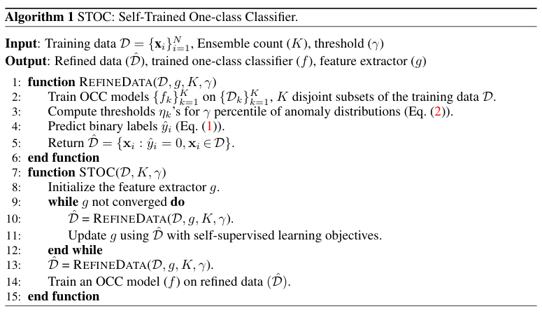
To this end, instead of training a single classifier, we train an ensemble of \(K\) one-class classifiers and aggregate their predictions to generate pseudo labels. We illustrate the data refinement block in Fig. 3 and as REFINEDATA in Algorithm 1. Specifically, we randomly divide the unlabeled training data \(\mathcal{D}\) into \(K\) disjoint subsets \(\mathcal{D}_1, \ldots, \mathcal{D}_K\), and train \(K\) different one-class classifiers \((f_1, \ldots, f_K)\) on corresponding subsets \((\mathcal{D}_1, \ldots, D_K)\). Then, we predict a binary label of the data \(\mathbf{x}_i \in D\) as follows:

$$ {\hat{y}}_{i}=1-\prod_{k=1}^{K}\left[1-\mathbf{1}\left(f_{k}(g(\mathbf{x}_{i}))\geq\eta_{k}\right)\right] $$ $$ \eta_{k}=\operatorname*{max}\eta {\quad\mathrm{s.t.}}\;{\frac{1}{N}}\sum_{i=1}^{N}\,\mathbf{1}(f_{k}(g({\bf x}_{i}))\ge\eta)\ge\gamma $$

where \(\mathbf{1}(\cdot)\) is the indicator function that outputs \(1/0\) if the input is True/False. \(f_k(g(\mathbf{x}_i))\) represents an anomaly score of \(\mathbf{x}_i\) for a one-class classifier \(f_k\). \(\eta_k\) in Eq. (2) is a threshold determined as a \(\gamma\) percentile of the anomaly score distribution \(\{f_k(g(\mathbf{x}_i))\}^N_{i=1}\).

Here \(\mathbf{x}_i\) is predicted as normal, i.e., \(\hat{y}_i = 0\), if all \(K\) one-class classifiers predict it as normal. While this may be too strict and potentially reject many true normal samples in the training set, we find that in practice it is more critical to be able to exclude true anomalous samples from the training set. The effectiveness of the ensemble classifier is empirically shown in Section 4.3.

Representation Update Link to heading

STOC follows the idea of deep representation one-class classifiers [41], where in the first stage deep neural network is trained with self-supervision, such as rotation prediction [20], contrastive [41], or CutPaste [28], to provide meaningful representations of the data, and in the second stage off-the-shelf one-class classifiers are trained on these learned representations. Such a two-stage framework is shown to be beneficial as it prevents the degeneracy of the deep one-class classifiers [36].

Here, we propose to conduct self-supervised representation learning jointly with the data refinement. More precisely, we train a trainable feature extractor \(g\) using \(\hat{\mathcal{D}} = \{\mathbf{x}_i : \hat{y}_i = 0\}\), a subset of unlabeled data \(\mathcal{D}\) that includes samples whose predicted labels with an ensemble one-class classifier are negative. We also update \(\hat{\mathcal{D}}\) as we proceed with the representation learning. The proposed method is illustrated in Algorithm 1 as STOC. In contrast to previous work [41, 28] that uses the entire training data for learning self-supervised representation, we find it necessary to refine the training data even for learning deep representations. Without representation refinement, the performance improvements of STOC are limited.

Following representation learning, we train a one-class classifier on refined data \(\hat{\mathcal{D}}\) using updated representation by \(g\) for test time prediction, as in lines 13, and 14 in Algorithm 1.

Selecting hyperparameters Link to heading

Our data refinement block introduces two hyperparameters: the number of one-class classifiers (\(K\)) and the percentile threshold (\(\gamma\)). First, there is a trade-off between the number of classifiers for the ensemble and the size of disjoint subsets for training each classifier. For example, with large \(K\), we aggregate prediction from many classifiers, each of which may contain more randomness. However, it comes at a cost of reduced performance per classifier as we use smaller subsets to train them. In practice, we find \(K = 5\) works well across different datasets and anomaly ratios in unlabeled training data. Second, \(\gamma\) controls the purity and coverage of refined data. If \(\gamma\) is large and thus classifiers reject too many samples, the refined data could be more pure and contain mostly the normal samples; however, the coverage of the normal samples would be limited. On the other hand, with small \(\gamma\), the refined data may still contain many anomalies and the performance improvement with STOC would be limited. As such, the performance of STOC could be suboptimal if the true anomaly ratio is not available. Nevertheless, in our experiments, we observe that STOC is robust to the selection of \(\gamma\) when chosen between the true anomaly ratio and the twice of that. This suggests that it is safer to use \(\gamma\) with an overestimate of true anomaly ratio.

Experiments Link to heading

Experiments on Tabular Domain Link to heading

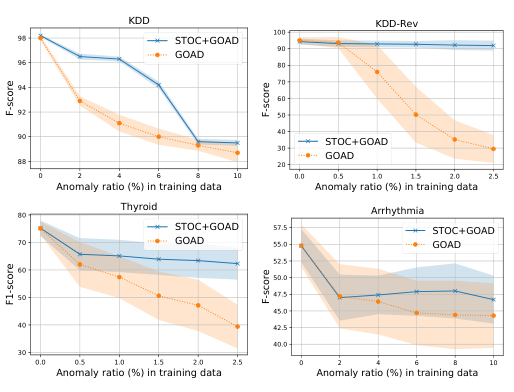
Datasets. Following [48, 5], we test the efficacy of STOC on a variety of tabular datasets, including KDDCup, Thyroid, or Arrhythmia from UCI repository [3]. We also use KDDCup-Rev, where the labels of KDDCup is reversed so that the attack represents an anomaly [48]. To construct data splits, we use \(50\%\) of normal samples for training. In addition, we take anomaly samples worthy of the \(10\%\) of the normal samples in the training set. This allows to simulate unsupervised settings with an anomaly ratio of up to \(10\%\) of the entire training set. The rest of the data is used for testing.1 We conduct experiments using \(5\) random splits and \(5\) random seeds. We report the average and standard deviation of \(25\) F1-scores (with a scale \(0-100\)) for the performance metric.

Models. We re-implement GOAD [5], a type of augmentation prediction method [19, 41] with random projections for learning representations, for the baseline with a few modifications. First, instead of using embeddings to compute the loss, we use a parametric classifier, similar to the augmentation prediction [41]. Second, we follow the two-stage framework [41] to construct deep one-class classifiers. For N setting, our implementation achieves \(98.0\) for KDD, \(95.0\) for KDD-Rev, \(75.1\) for Thyroid, and \(54.8\) for Arrhythmia F1-scores, which are comparable to those reported in [5].

Figure 4: Unsupervised anomaly detection performance (F1-score) using GOAD [5] and that with STOC on various tabular datasets. Shaded areas represent the standard deviation.

Experiments on Image Domain Link to heading

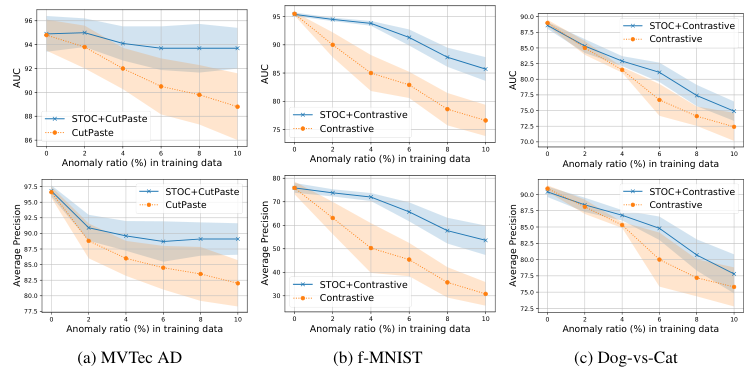
Datasets. We evaluate STOC on visual anomaly detection benchmarks, including CIFAR-10 [25], f-MNIST [44], Dog-vs-Cat [16], and MVTec anomaly detection (AD) [6]. For CIFAR-10, f-MNIST, and Dog-vs-Cat datasets, samples from one class are set to be normal and the remainders from other classes are set to be anomaly. Similarly to experiments on tabular data, we swap a certain amount of the normal training data with anomalies so that the anomaly ratio reaches the target percentage for unsupervised settings. For MVTec AD experiments, since there is no anomalous data available for training, we borrow \(10\%\) of the anomalies from the test set and swap them with normal samples in the training set. Note that the \(10\%\) of samples borrowed from the test set are excluded from evaluation. For all datasets, we experiment with varying anomaly ratios from \(0\%\) to \(10\%\). We use area under ROC curve (AUC) and average precision (AP) metrics to quantify the performance of visual anomaly detection (with scale \(0-100\)). When computing AP, we set the minority class of the test set as label \(1\) and majority as label \(0\) (e.g., normal samples are set as label \(1\) for CIFAR-10 experiments as there are more anomaly samples that are from \(9\) classes in the test set). We run all experiments with 5 random seeds, and report the average performance for each dataset across all classes in Fig. 5 and Fig. 6.

Models. For semantic anomaly detection benchmarks, CIFAR-10, f-MNIST, and Dog-vs-Cat, we compare the STOC with two-stage one-class classifiers [41] using various representation learning methods, such as distribution-augmented contrastive learning [41], rotation prediction [19, 20] and its improved version [41], or denoising autoencoder. For MVTec AD benchmarks, we use CutPaste [28] as a baseline and compare to its version with STOC integration. For both experiments, we use ResNet-18 model, trained from random initialization, using the hyperparameters from [41] and [28]. The same model and hyperparameter configurations are used for STOC with \(K = 5\), the count of classifier ensembles. We set \(\gamma\) as twice the anomaly ratios of the training data. For \(0\%\) anomaly ratios, we set \(\gamma\) as \(0.5\). Finally, Gaussian Density Estimator (GDE) on learned representations is used for one-class classifiers.

Figure 5: Unsupervised anomaly detection performance with various one-class classifiers on CIFAR- 10 dataset. For STOC we adopt distribution-augmented contrastive representation learning [41]. (Left) AUC, (Right) Average Precision (AP).

Figure 6: Unsupervised anomaly detection performance on (a) MVTec AD (b) f-MNIST, and (c) Dog-vs-Cat datasets with varying anomaly ratios. We use state-of-the-art one-class classification models for baselines, such as distribution-augmented contrastive representations [41] for f-MNIST and Dog-vs-Cat, or CutPaste [28] for MVTec AD, and build STOC on top of them.

Conclusion Link to heading

Anomaly detection has wide range of practical use cases. A challenging and costly aspect of building an anomaly detection system is labeling as anomalies are rare and are not easy to detect by humans. To enable high-performance anomaly detection without any labels, we propose a novel anomaly detection framework, STOC. STOC can be flexibly integrated with any one-class classifier, applied on raw data or on trainable representations. STOC employs an ensemble of multiple one-class classifiers to propose candidate anomaly samples that are refined from training, which allows more robust fitting of the anomaly decision boundaries as well as better learning of data representations. We demonstrate the state-of-the-art anomaly detection performance of STOC on multiple tabular and image data.

STOC has the potential to make huge positive impact in real-world AD applications where detecting anomalies is crucial, such as for financial crime elimination, cybersecurity advances, or improving manufacturing quality. We note the potential risk associated with using STOC that when representations are not sufficiently good, there will be a negative cycle of refinement and representation updates/one-class classifier. While we rely on the existence of good representations this may not be true for other domains (e.g., cybersecurity). This paper focuses on unsupervised setting, and demonstrates strong anomaly detection performance. This opens new horizons for human-in-the-loop anomaly detection systems that are low-cost and robust. We leave these explorations to future work.