Stichable Neural Networks

Abstract Link to heading

As each model family consists of pretrained models with diverse scales (e.g., DeiT-Ti/S/B), it naturally arises a fundamental question of how to efficiently assemble these readily available models in a family for dynamic accuracy-efficiency trade-offs at runtime.

The paper presents Stitchable Neural Networks (SN-Net), a novel scalable and efficient framework for model deployment. It cheaply produces numerous networks with different complexity and performance trade-offs given a family of pretrained neural networks, which are called anchors. Specifically, SN-Net splits the anchors across the blocks/layers and then stitches them together with simple stitching layers to map the activations from one anchor to another. With only a few epochs of training, SN-Net effectively interpolates between the performance of anchors with varying scales. At runtime, SN-Net can instantly adapt to dynamic resource constraints by switching the stitching positions.

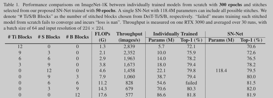
Extensive experiments on ImageNet classification demonstrate that SN-Net can obtain on-par or even better performance than many individually trained networks while supporting diverse deployment scenarios.

Introduction Link to heading

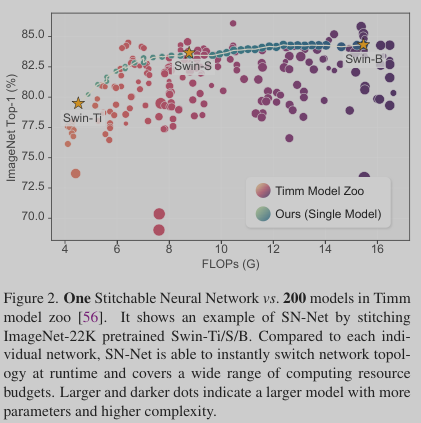
Up to now, there are ∼81k models on HuggingFace and ∼800 models on Timm that are ready to be downloaded and executed without the overhead of reproducing. Despite the large model zoo, a model family (e.g., DeiT-Ti/S/B) that contains pretrained models with functionally similar architectures but different scales only covers a coarse-grained level of model complexity/performance, where each model only targets a specific resource budget (e.g., FLOPs). Moreover, the model family is not flexible to adapt to dynamic resource constraints since each individual model is not re-configurable due to the fixed computational graph.

In reality, we usually need to deploy models to diverse platforms with different resource constraints (e.g., energy, latency, on-chip memory). For instance, a mobile app in Google Play has to support tens of thousands of unique Android devices, from a high-end Samsung Galaxy S22 to a low-end Nokia X5. Therefore, given a family of pretrained models in the model zoo, a fundmental research question naturally arises: how to effectively utilise these off-the-shelf pretrained models to handle diverse deployment scenarios for Green AI

A naive solution is to train individual models with different accuracy-efficiency trade-offs from scratch. However, such method has a linearly increased training and time cost with the number of possible cases. Therefore, one may consider the existing scalable deep learning frameworks, such as model compression and neural architecture search (NAS), to obtain models at different scales for diverse deployment requirements

Network compression approaches such as pruning, quantization and knowledge distillation aim to obtain a small model from a large and well-trained network, which however only target one specific resource budget, thus not flexible to meet the requirements of real-world deployment scenarios.

One-shot NAS, a typical NAS framework that decouples training and specialization stages, seeks to train an over-parameterized supernet that supports many sub-networks for run-time dynamics, but training the supernet is extremely timeconsuming and computationally expensive.

To summarize, the existing scalable deep learning frameworks are still limited within a single model design space, which cannot inherit the rich knowledge from pretrained model families in a model zoo for better flexibility and accuracy.

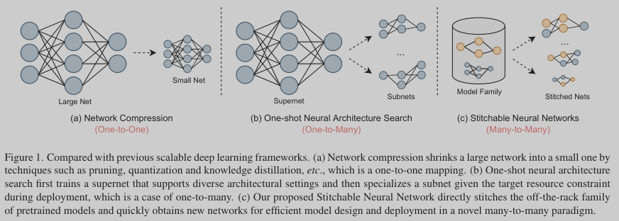
The authors present Stitchable Neural Network (SN-Net), a novel scalable deep learning framework for efficient model design and deployment which quickly stitches an off-the-shelf pretrained model family with much less training effort to cover a fine-grained level of model complexity/performance for a wide range of deployment scenarios. Specifically, SN-Net is motivated by the previous observations that the typical minima reached by SGD can be stitched to each other with low loss penalty, which implies architectures of the same model family pretrained on the same task can be stitched.

Based on this insight, SN-Net directly selects the well-performed pretrained models in a model family as “anchors”, and then inserts a few simple stitching layers at different positions to transform the activations from one anchor to its nearest anchor in terms of complexity. In this way, SN-Net naturally interpolates a path between neighbouring anchors of different accuracy-efficiency trade-offs, and thus can handle dynamic resource constraints with a single neural network at runtime.

Model Stiching Link to heading

Model stitching was initially proposed by Lenc et al. to study the equivalence of representations. Specifically, they showed that the early portion of a trained network can be connected with the last portion of another trained network by a 1 x 1 convolution stitching layer without significant performance drop. Most recently, Yamini et al. revealed that neural networks, even with different architectures or trained with different strategies, can also be stitched together with small effect on performance. As a concurrent work, Adrian et al. studied using model stitching as an experimental tool tomatch neural network representations.

Neural Architecture Search. Link to heading

Neural architecture search (NAS) aims to automatically search for the well- performed network architecture in a pre-defined search space under different resource constraints. In the early attempts, NAS consumes prohibitive computational cost due to the requirement of training individual sub-networks until convergence for accurate performance estimation. To address this problem, one-shot NAS has been proposed to improve NAS efficiency by weight sharing, where multiple subnets share the same weights with the supernet. However, training a supernet still requires intensive computing resources. Most recently, zero-shot NAS has been proposed to identify good architectures prior to training. However, obtaining the final ing from scratch.

Method Link to heading

Preliminaries Link to heading

Let $\theta$ be the model parameters of a pretrained neural network and $f_{i}$ represent the function of the $i$-th layer. A typical feed-forward neural network with $L$ layers can be defined as a composition of functions: $f_{\theta} = f_{L} \circ \ldots \circ f_{1}$, where $\circ$ indicates the composition, and $f_{\theta} : X \rightarrow Y$ maps the inputs in an input space $X$ to the output space $Y$. Let $X \in X$ be an input to the network.

The basic idea of model stitching involves splitting a neural network into two portions of functions at a layer index $l$. The first portion of layers compose the front part that maps the input X into the activation space of the $l$-th layer $\mathcal{A}_{\theta},l$, which can be formulated as

$$H_{\theta,l}(\mathbf{X}) = f_{l} \circ \ldots \circ f_{1}(\mathbf{X}) = \mathbf{X}_{l}$$

where $\mathbf{X}_{l} \in \mathcal{A}_{\theta, l}$ denotes the output feature map at the $l$-th layer. Next, the last portion of layers maps

$$\mathbf{X}_{l}$$

into the final output

$$T_{\theta,l}(\mathbf{X}) = f_{L} \circ \ldots \circ f_{l+1}(\mathbf{X})$$

In this case, the original neural network function $f_{\theta}$ can be defined as a composition of the above functions $f_{\theta} = T_{\theta,l} \circ H_{\theta,l}$ for all layer indexes $l = 1, \ldots, L−1$.

Now suppose we have another pretrained neural network $f_{\phi}$. Let $\mathcal{S} : \mathcal{A}_{\theta,l} \rightarrow \mathcal{A}_{\phi, m}$ be a stitching layer which implements a transformation between the activation space of the $l$-th layer of $f_{\theta}$ to the activation space of the $m$-th layer of $f_{\phi}$. The basic idea of model stitching to obtain a new network defined by $\mathcal{S}$ can be expressed as

$$F_S(\mathbf{X}) = T_{\phi,m} \circ \mathcal{S} \circ H_{\theta,l}(\mathbf{X})$$

By controlling the stitched layer indexes $l$ and $m$, model stitching can produce a sequence of stitched networks. Models of the same architecture but with different initializations (i.e., random seeds) can be stitched together with low loss penalty. Different architectures (e.g., ViTs and CNNs) may also be stitched without significant performance drop.

Stitchable Neural Networks Link to heading

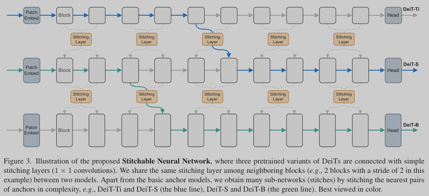
Stitchable Neural Networks (SN-Net), a new “many-to-many” elastic model paradigm. SN-Net is motivated by an increasing number of pretrained models in the publicly available model zoo, where most of the individually trained models are not directly adjustable to dynamic resource constraints. To this end, SN-Net inserts a few stitching layers to smoothly connect a family of pretrained models to form diverse stitched networks permitting run-time network selection. The framework of SN-Net is illustrated in Figure 3 by taking plain ViTs as an example. For brevity, we will refer to the models that to be stitched as “anchors” and the derived models by stitching anchors as “stitches”.

What to stitch: the choice of anchors. In general, the large-scale model zoo determines the powerful representation capability of SN-Net as it is a universal framework for assembling the prevalent families of architectures. SN-Net works for stitching representative ViTs and CNNs. However, intuitively, anchors that are pretrained on different tasks can learn very different representations (e.g., ImageNet and COCO) due to the large distribution gap of different domains, thus making it difficult for stitching layers to learn to transform activations among anchors. Therefore, the selected anchors should be consistent in terms of the pretrained domain.

How to stitch: the stitching layer and its initialization. Conceptually, the stitching layer should be as simple as possible since its aim is not to improve the model performance, but to transform the feature maps from one activation space to another. To this end, the stitching layers in SN-Net are simply 1 × 1 convolutional layers. By default in PyTorch, these layers are initialized based on Kaiming initialization.

SN-Net is built upon pretrained models. In this case, the anchors have already learned good representations, which allows to directly obtain an accurate transformation matrix by solving the following least squares problem

$$||\mathbf{A}\mathbf{M}_{o} - \mathbf{B}||_{F} = \mathrm{min}||\mathbf{A}\mathbf{M} - \mathbf{B}||_{F}$$

where $\mathbf{A} \in \mathbb{R}^{N \times D_1}$, $\mathbf{B} \in \mathbb{R}^{N \times D_2}$ are two feature maps of the same spatial size but with different number of hidden dimensions. N denotes the length of the input sequence and $D_1$, $D_2$ refer to the number of hidden dimensions. $\mathbf{M} \in \mathbb{R}^{D_1 \times D_2}$ is the targeted transformation matrix.

Optimal solution can be achieved through an orthogonal projection in the space of matrices

$$\mathbf{M}_o = \mathbf{A}^\dagger\mathbf{B}$$

where $\mathbf{A}^\dagger$ denotes the Moore-Penrose pseudoinverse of $\mathbf{A}$. To obtain $\mathbf{M}_o$ requires only a few seconds on one CPU with hundreds of samples.

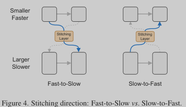
Where to stitch: the stitching directions. Given anchors with different scales and complexities, there are two options to stitch them together: Fast-to-Slow and Slow-to-Fast. Taking two anchors as an example (Figure 4), Fast-to-Slow takes the first portion of layers (i.e., Eq. (1)) from a smaller and faster model, and the last portion of layers (i.e., Eq. (1)) from a larger and slower model, where Slow-to-Fast goes in a reverse direction. However, as Fast-to-Slow is more aligned with the existing model design principle (i.e., increasing the network width as it goes deeper), it achieves more stable and better performance than Slow-to-Fast. In this case, we take Fast-to-Slow as the default stitching direction in SN-Net. Besides, as different anchors may reach very different minima, we propose a nearest stitching strategy by limiting the stitching between two anchors of the nearest model complexity/performance.

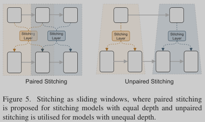
Way to stitch: stitching as sliding windows. Our stitching strategy is inspired by the main observation: neighboring layers dealing with the same scale feature maps share similar representations. To this end, we propose to stitch anchors as sliding windows, where the same window

shares a common stitching layer, as shown in Figure 5. Let $L_1$ and $L_2$ be depth of two anchors. Then intuitively, there are two cases when stitching layers/blocks between the two anchors: paired stitching ($L_1 = L_2$) and unpaired stiching ($L_1 \neq L_2$). In the case of $L_1 = L_2$, the sliding windows can be controlled as sliding windows with a window size $k$ and a stride $s$. Figure 5 left shows an example with $k = 2$, $s = 1$. However, in most cases we have unequal depth as different model architectures have different scales.

Stitching Space. In SN-Net, we first split the anchors along the internal layers/blocks at each stage then apply our stitching strategy within each stage. As different anchors have different architectural configurations, the size of the stitching space can be variant based on the depth of the selected anchors and the stitching settings (i.e., the kernel size $k$ and stride $s$). More stitches can be obtained by choosing anchors with larger scales or configuring the sliding windows by using a larger window size or smaller stride. Overall, compared to one-shot NAS which can support more than 1020 sub-networks, SN-Net has a relatively smaller space (up to hundreds or thousands). However, we point out that even though NAS has a much larger architecture space, during deployment, it only focuses on the sub-networks on the Pareto frontier of performance and resource consumption.

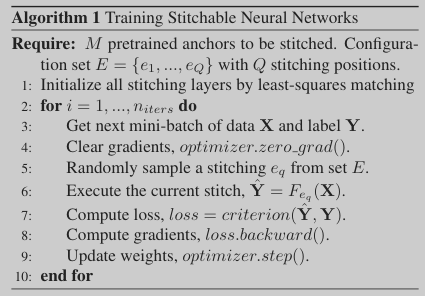
Training strategy. Given the anchors with different accuracy-efficiency trade-offs from the model zoo, our aim is to train an elastic joint network that covers a large num- ber of stitches in a highly efficient way so that it can fit diverse resource constraints with low energy cost.